Excel Tutorial - How to use Pivot Tables

Create a PivotTable to analyze worksheet data – Excel

Being able to analyze all the data in your worksheet can help you make better business decisions. But sometimes it’s hard to know where to start, especially when you have a lot of data. Excel can help you by recommending and then automatically creating PivotTables, which are a great way to summarize, analyze, explore, and present your data.

Make sure your data has column headings or table headers, and that there are no blank rows.
Click any cell in the range of cells or table.
Click Insert > Recommended PivotTables.
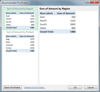
In the Recommended PivotTables dialog box, click any PivotTable layout to get a preview, and then pick the one that shows the data the way you want.
Click OK.Excel places the PivotTable on a new worksheet and shows the Field List so you can further rearrange the PivotTable data as needed.
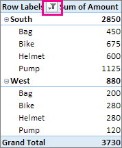
To zero in on the data and arrange it the way you want, you can filter and sort the PivotTable. See Filter data in a PivotTable and Sort data in a PivotTable.In the example shown below, Row Labels is filtered to show only sales for the South and West regions.